Introduction
IntroductionImagine you and your friend are driving on a highway in two separate cars, and you want to follow your friend's car at about 50 meters behind. You can observe your distance to your friend's car (e.g., far, close, or okay), and your relative speed to it (e.g., fast, slow, or okay). Then, how would you adjust your acceleration (gas pedal), so that the distance is kept at roughly 50 meters?
Some intuitive rules would apply, e.g.,
$\mbox{IF the distance is far AND your relative speed is slow, THEN your acceleration should be positive};$
$\mbox{IF the distance is close AND your relative speed is fast, THEN your acceleration should be negative};$
$\mbox{IF the distance is okay AND your relative speed is okay, THEN your acceleration should be about zero};$
and so on. A human driver can adjust the acceleration intuitively, without using any mathematics.
Then, how about designing a car following controller for this task? How would you transform the above knowledge (rules) into mathematical formulas, so that the controller can calculate the appropriate acceleration based on the distance and speed?
Fuzzy systems are in this regard very suitable tools. Next, we will introduce how they can be used to solve this problem.
Type-1 Fuzzy Sets and Fuzzy Systems
Type-1 Fuzzy Sets and Fuzzy SystemsA. Type-1 Fuzzy Sets
Type-1 Fuzzy SetsType-1 (T1) fuzzy set was first introduced by Zadeh
Definition 1
Type-1 Fuzzy Sets Definition 1equation1 A T1 fuzzy set $X$ is comprised of a domain $D_X$ of real numbers (also called the universe of discourse of $X$) together with a membership function (MF) $u_{_X}(x):\ D_X \to [0,1]$, i.e.,
$X=\int_{D_X}u_{_X}(x)/x .$ $(1)$
$(1)$ is a fuzzy set notation, introduced by Zadeh, as a shorthand in which $\int$ denotes the collection of all points $x\in D_X$ with associated membership grade $u_{_X}(x)$.

The membership grade of $x$ can be computed as:
$u_X(x)=\left\{\begin{array}{cl} \frac{x-a}{b-a}, & x\in(a,b) \\ 1, & x\in[b,c] \\ \frac{d-x}{d-c}, & x\in(c,d)\\ 0, & \mbox{otherwise} \end{array}\right .$$(2)$
A triangular T1 fuzzy set is a special case of a trapezoidal T1 fuzzy set, when $b=c$.
Figure $2$ shows a specific example of a T1 fuzzy set "Moderate". When only integer numbers are considered in the domain, the T1 fuzzy set can be represented as $\{0/1, 0.5/2, 1/3, 1/4, 0.5/5, 0/6\}$, where $0/1$ means that $x=1$ has a membership grade of 0 in Moderate, and $0.5/2$ means $x=2$ has a membership grade of $1$ in Moderate. Figure $2$ shows that there is a complete agreement (certainty) for $x\in[0,1]\cup[3,4]\cup[6,+\infty)$, and a partial agreement for $x\in(1,3)\cup(4,6)$. In contrast, for a crisp set, the membership grade of each element in it is either 0 or 1; there is no value (e.g., 0.3) in between, i.e., a crisp set cannot model a partial agreement.
Figure 2Try to drag the blue dot and change the membership grade of $x$.
|
B. T1 Fuzzy System
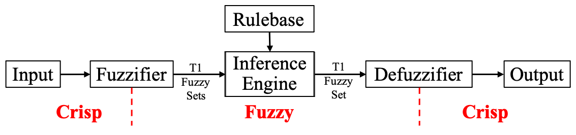
Type-1 Fuzzy SystemsFigure $3$ shows the diagram of a typical T1 fuzzy system, which consists of four components: fuzzifier, rulebase, inference engine, and defuzzifier. The fuzzifier transforms crisp inputs into T1 fuzzy sets. The inference engine performs inference on the T1 fuzzy sets, combining the outputs of the rules in the rulebase into a new T1 fuzzy set. The defuzzifier converts the mapped T1 fuzzy set into a crisp output.
There are two kinds of rules for fuzzy systems, Zadeh (Mamdani), in which rule consequents are
words modeled by T1 fuzzy sets
T1 TSK rules are:
$R_k: \mbox{ IF } X_1 \mbox{ is } X_{k,1} \mbox{ AND } \cdots \mbox{ AND } X_d \mbox{ is } X_{k,d}, \mbox{ THEN } y_k(\mathbf{x}) = \sum_{i=1}^d a_{k,i}x_i + b_k, \quad k=1,...,K$
where $d$ is the input dimensionality, $K$ is the number of rules, $X_{k,i}$ is a linguistic term (modeled by a T1 fuzzy set) for linguistic variable $X_i$ ($i=1,...,d$) in the $k^{\mathrm{th}}$ rule, $x_i$ is the crisp input for $X_i$, and $a_{k,i}$ and $b_k$ ($k=1,...,K$) are adjustable regression coefficients. Many times all $a_{k,i}$ are set to 0, i.e., each rule consequent is a constant.
For the car following example, $d=2$, $X_1$ denotes Distance, $X_2$ denotes Relative Speed, $K=9$ if both Distance and Relative Speed have three linguistic terms (T1 fuzzy sets), and $x_1$ and $x_2$ are the current input values of Distance and Relative Speed, respectively.
For a particular input $\mathbf{x}=(x_1,...,x_d)$, the operations in a TSK fuzzy system are:
-
Fuzzification:
Compute $u_{X_{k,i}}(x_i)$, the membership grade of $x_i$ on $X_{k,i}$ ($k=1,...,K$; $i=1,...,d$).
-
Inference:
Compute the firing level of each rule:
$f_k(\mathbf{x})=u_{X_{k,1}}(x_1)\times\cdots\times u_{X_{k,d}}(x_d),$
Units $y(\mathbf{x})=\frac{\sum_{k=1}^K f_k(\mathbf{x})\cdot y_k(\mathbf{x})}{\sum_{k=1}^K f_k(\mathbf{x})}.$ $(3)$
Note that the minimum operation could also be used to replace the multiplication above. The inference engine output is: -
Defuzzification:
Since the inference output is already a crisp number, no defuzzification is needed in a T1 TSK fuzzy system. The inference output $y(\mathbf{x})$ is the final output.
However, for Mamdani T1 fuzzy systems, since the rule consequents are words modeled by T1 fuzzy sets, the inference output is also a T1 fuzzy set, which must be defuzzified to obtain a crisp output. One popular defuzzification approach is to compute the centroid of that T1 fuzzy set.
$(3)$ fuses the consequents of multiple rules to give an output. If we view each rule as an expert,
then a TSK fuzzy system is functionally equivalent to a mixture of expert model
C. Car Following Example
Type-1 Fuzzy exampleThis subsection presents a simple example to illustrate the computations in a T1 TSK fuzzy system. Consider the car following example introduced at the beginning of this paper.
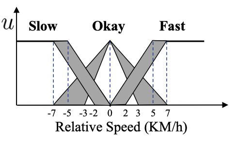
Assume the distance has three linguistic terms (modeled by T1 fuzzy sets), Close, Okay and Far, as depicted in Figure $4(a)$, and the relative speed also has three linguistic terms (modeled by T1 fuzzy sets), Slow, Okay and Fast, as depicted in Figure $4(b)$. Note that the same word "Okay" for the distance and the relative speed could have different T1 FS definitions.
Figure4(a) Figure4(b)

T1 fuzzy sets for the distance and the relative speed, in the car following example.
There are nine rules, whose consequents are crisp numbers:
-
$R_1: \mbox{ IF distance is Close AND relative speed is Slow, THEN acceleration is } y_1=0$
-
$ R_2: \mbox{ IF distance is Close AND relative speed is Okay, THEN acceleration is } y_2=-5 $
-
$ R_3: \mbox{ IF distance is Close AND relative speed is Fast, THEN acceleration is } y_3=-10$
-
$R_4: \mbox{ IF distance is Okay AND relative speed is Slow, THEN acceleration is } y_4=3$
-
$R_5: \mbox{ IF distance is Okay AND relative speed is Okay, THEN acceleration is } y_5=0$
-
$R_6: \mbox{ IF distance is Okay AND relative speed is Fast, THEN acceleration is } y_6=-3$
-
$R_7: \mbox{ IF distance is Far AND relative speed is Slow, THEN acceleration is } y_7=10$
-
$R_8: \mbox{ IF distance is Far AND relative speed is Okay, THEN acceleration is } y_8=5$
-
$R_9: \mbox{ IF distance is Far AND relative speed is Fast, THEN acceleration is } y_9=0$
Assume the current distance to the front car is 47 meters, and the relative speed is 4 KM/h. The membership grades of the corresponding T1 fuzzy sets are shown in Figure $5$:
$\quad u_{_{\mathrm{Close}}}($
$\quad u_{_{\mathrm{Slow}}}($
Try to drag the dots to change the distance and relative speed values.
The membership grades and all subsequent calculations will be updated accordingly.
|
Membership grades on the T1 fuzzy sets. (a) Distance is meters, the membership interval on Close is , on Okay is , and on Far is ; (b) Relative speed is KM/h, the membership interval on Slow is , on Okay is , and on Fast is .
The firing levels of the nine rules are:
-
$R_1: \quad f_1($
$, $ $)\quad=\quad u_{_{\mathrm{Close}}}($ $) \quad\times \quad u_{_{\mathrm{Slow}}}($ $)\quad= \quad$ $\quad\times\quad$ $\quad=\quad$ -
$R_2: \quad f_2($
$, $ $)\quad=\quad u_{_{\mathrm{Close}}}($ $) \quad\times \quad u_{_{\mathrm{Okay}}}($ $)\quad= \quad$ $\quad\times\quad$ $\quad=\quad$ -
$R_3: \quad f_3($
$, $ $)\quad=\quad u_{_{\mathrm{Close}}}($ $) \quad\times\quad u_{_{\mathrm{Fast}}}($ $)\quad= \quad$ $\quad\times\quad$ $\quad=\quad$ -
$R_4: \quad f_4($
$, $ $)\quad=\quad u_{_{\mathrm{Okay}}}($ $)\quad \times \quad u_{_{\mathrm{Slow}}}($ $)\quad= \quad$ $\quad\times\quad$ $\quad=\quad$ -
$R_5: \quad f_5($
$, $ $)\quad=\quad u_{_{\mathrm{Okay}}}($ $)\quad \times \quad u_{_{\mathrm{Okay}}}($ $)\quad= \quad$ $\quad\times\quad$ $\quad=\quad$ -
$R_6: \quad f_6($
$, $ $)\quad=\quad u_{_{\mathrm{Okay}}}($ $) \quad\times \quad u_{_{\mathrm{Fast}}}($ $)\quad=\quad $ $\quad\times\quad$ $\quad=\quad$ -
$R_7: \quad f_7($
$, $ $)\quad=\quad u_{_{\mathrm{Far}}}($ $)\quad \times \quad u_{_{\mathrm{Slow}}}($ $)\quad=\quad $ $\quad\times\quad$ $\quad=\quad$ -
$R_8: \quad f_8($
$, $ $)\quad=\quad u_{_{\mathrm{Far}}}($ $)\quad \times\quad u_{_{\mathrm{Okay}}} ($ $)\quad= \quad$ $\quad\times\quad$ $\quad=\quad$ -
$R_9: \quad f_9($
$, $ $)\quad=\quad u_{_{\mathrm{Far}}}($ $)\quad \times \quad u_{_{\mathrm{Fast}}}($ $)\quad=\quad $ $\quad\times\quad$ $\quad=\quad$
The output acceleration is:
equation1 $\quad($$\quad=\quad[$
$\quad\quad\quad\div $ $\quad [$
$\quad=\quad$
i.e., the car should have to maintain the distance at 50 meters.
This is intuitive, as the current distance 50 meters, and the relative speed .
The above nine rules are summarized in Table $ 1$. The corresponding input-output mapping is shown in Figure $6$, which can be changed by modifying the rule consequents in Table $1$.
Rulebase of the T1 TSK fuzzy system in the car following example. The numbers are rule consequents, i.e., acceleration (KM/h$^2$). Any numbers can be used for rule consequents, and the T1 TSK fuzzy system can always give an output. However, the suggested range is [-10, 10]. For reasonableness, the rule consequents in the same row should increase from the left to the right, e.g., when Distance is Close, as Relative Speed increases, Acceleration should become more negative, i.e., $y_1\leq y_2\leq y_3$. The rule consequents in the same column should increase from the top to the bottom, e.g., when Relative Speed is Slow, as Distance increases, Acceleration should also increase, i.e., $y_1\leq y_4\leq y_7$.
| Distance$\setminus$Relative Speed | Slow | Okay | Fast |
|---|---|---|---|
| Close | $y_1=$ | $y_2=$ | $y_3=$ |
| Okay | $y_4=$ | $y_5=$ | $y_6=$ |
| Far | $y_7=$ | $y_8=$ | $y_9=$ |
Figure 6
Try to change the rule consequent values in Table $ 1$ by direct typing or clicking on the sidebar arrows.
After adjusting the rulebase, click the "Update" button to update all calculations.
|
Input-output mapping of the T1 fuzzy system. The figure can be zoomed and rotated by using the mouse or the top right buttons.
Interval Type-2 Fuzzy Sets and Fuzzy Systems
Interval Type-2 (IT2) Fuzzy Sets and Fuzzy Systems
Despite having a name which carries the connotation of uncertainty,
research has shown that there are limitations in the ability of T1 fuzzy sets to model
and minimize the effect of uncertainties
For example, different drivers may have different understanding of the linguistic term Far in the motivating example,
and hence may provide different T1 fuzzy sets for it.
Type-2 fuzzy sets
A. IT2 Fuzzy Sets
IT2 Fuzzy SetsInterval type-2 (IT2) fuzzy sets
Definition 2
IT2 fuzzy set Definition 2
An IT2 fuzzy set $\tilde{X}$ is defined as
equation1 $\widetilde{X}=\int\limits_{x\in D_{\tilde{X}}}\,\int\limits_{u\in [0,1]}1/(x,u) =\int\limits_{x\in D_{\tilde{X}}}\left.\left[\int\limits_{u\in [0,1]}1/u\right]\right/x$ $(5)$where $x$, called the primary variable, is in domain $D_{\tilde{X}}$; $u\in [0,1]$ is the secondary variable; and, the secondary grade of $\tilde{X}$ equals 1 for $\forall x\in D_{\tilde{X}}$ and $\forall u\in [0,1]$.
An example of an IT2 fuzzy set $\tilde{X}$ is shown in Figure $7$. Observe that unlike a T1 fuzzy set, whose membership for each $x$ is a number, the membership of an IT2 fuzzy set is an interval. For example, the membership of $x=3$ is $[0.25, 1]$, and the membership of $x=5$ is $[0.75, 1]$. A membership interval $[0.25, 1]$ means that some people think the membership of $x=3$ is $0.25$, some think the membership is $1$, and others may think the membership is any value between $0.25$ and $1$, i.e., an IT2 fuzzy set can model inter-personal uncertainties, whereas a T1 fuzzy set cannot.
Figure $7$ shows that an IT2 fuzzy set is bounded from the above and below by two T1 fuzzy sets, which are called upper MF (UMF) and lower MF (LMF). The area between the LMF and the UMF is the footprint of uncertainty (FOU).
Try to drag the blue or green dot to change the membership interval of $x$.
|
Example of an IT2 fuzzy set. When the input x= , the membership interval is [, ], represented by the red dashed line.
B. IT2 Fuzzy System
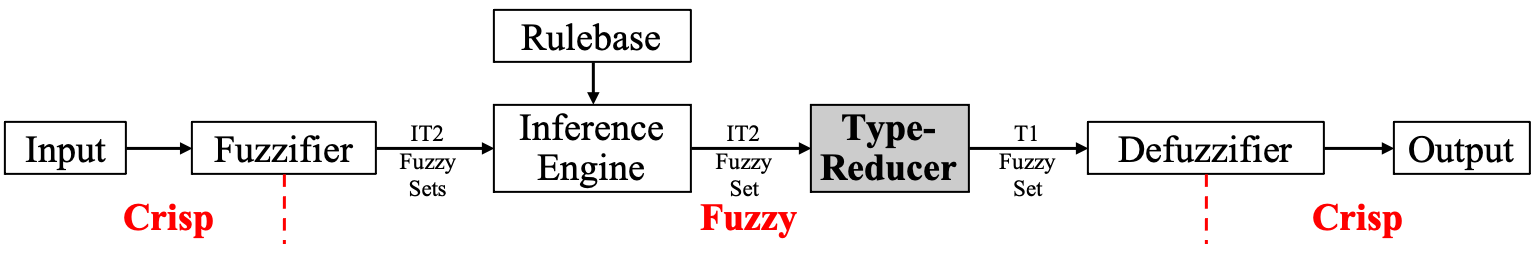
IT2 Fuzzy SystemFigure $8$ shows the schematic diagram of an IT2 fuzzy system. It is similar to its T1 counterpart, with
the major difference being that at least one of the fuzzy sets in the rulebase is an IT2 fuzzy set.
Hence, the outputs of the inference engine are IT2 fuzzy sets, and a type-reducer is usually needed
(it can be bypassed
An IT2 fuzzy system.
Assume the rulebase of an IT2 TSK fuzzy system consisting of $K$ rules in the following form:
$\tilde{R}_k: \mbox{ IF } x_1 \mbox{ is } \widetilde{X}_{k,1} \mbox{ AND } \cdots \mbox{ AND } x_d \mbox{ is } \widetilde{X}_{k,d}, \mbox{ THEN } Y_k(\mathbf{x}) = [\underline{y}_k,\ \overline{y}_k], \quad k=1,...,K $
where $\widetilde{X}_{k,i}$ $(i=1,\ldots,d)$ are IT2 fuzzy sets,
and $Y_k(\mathbf{x}) = [\underline{y}_k,\ \overline{y}_k]$ is an interval,
which can be understood as the centroid
For a particular input $\mathbf{x}=(x_1,...,x_d)$, the output of the IT2 TSK fuzzy system is computed as:
-
Fuzzification:
Compute the membership interval $[u_{\underline{X}_{k,i}}(x_i),u_{\overline{X}_{k,i}}(x_i)]$ of $x_i$ on each $\widetilde{X}_{k,i}$ ($k=1,...,K$; $i=1,...,d$).
-
Inference:
Compute the firing interval of the $k^{\mathrm{th}}$ rule, $F_k(\mathbf{x})$:
equation1$F_k (\mathbf{x}) = [u_{\underline{X}_{k,1}}(x_1)\times\cdots\times u_{\underline{X}_{k,d}}(x_d), u_{\overline{X}_{k,1}}(x_1)\times\cdots\times u_{\overline{X}_{k,d}}(x_d)] \equiv [\underline{f}_k,\,\overline{f}_k], \quad k=1,...,K$ $(6)$
Note that the minimum operation could also be used to replace the multiplication above. Inference is performed by:
$Y(\mathbf{x}) = \bigcup\limits_{f_k \in F_k(\mathbf{x}) \atop y_k \in Y_k(\mathbf{x})} \frac{\sum\limits_{k=1}^K f_k y_k} {\sum\limits_{k=1}^K f_k}. $ $(7)$
$(7)$is a direct extension of $(3)$, when all $f_k(\mathbf{x})$ and $y_k(\mathbf{x})$ in $(3)$ become intervals.
-
Type-reduction:
Many different approaches
can be used to compute $(7)$. When the popular center-of-sets type-reducer is used, the type-reduced output is: $ Y(\mathbf{x}) =[y_l,\ y_r],$ $(8)$
where:
$y_l=\min\limits_{l\in[1,K-1]}\frac{\sum_{k=1}^l\overline{f}_k\underline{y}_k+\sum_{k=l+1}^K \underline{f}_k\underline{y}_k} {\sum_{k=1}^l\overline{f}_k+\sum_{k=l+1}^K\underline{f}_k}\equiv \frac{\sum_{k=1}^L\overline{f}_k\underline{y}_k+\sum_{k=L+1}^K\underline{f}_k\underline{y}_k} {\sum_{k=1}^L\overline{f}_k+\sum_{k=L+1}^K\underline{f}_k}, $ $(9)$
$ y_r=\max\limits_{r\in[1,K-1]}\frac{\sum_{k=1}^r\underline{f}_k\overline{y}_k+\sum_{k=r+1}^K \overline{f}_k\overline{y}_k} {\sum_{k=1}^r\underline{f}_k+\sum_{k=r+1}^K\overline{f}_k}\equiv \frac{\sum_{k=1}^R\underline{f}_k\overline{y}_k+\sum_{k=R+1}^K\overline{f}_k\overline{y}_k} {\sum_{k=1}^R\underline{f}_k+\sum_{k=R+1}^K\overline{f}_k}, $ $(10)$
in which the switch points $L$ and $R$ are determined by
$ \underline{y}_L \le y_l\le \underline{y}_{L+1},$ $(11)$
$ \overline{y}_R \le y_r\le \overline{y}_{R+1},$ $(12)$
and $\{\underline{y}_k\}_{k=1}^K$ and $\{\overline{y}_k\}_{k=1}^K$ have been sorted in ascending order, separately.
$y_l$ and $y_r$ can be computed using the original Karnik-Mendel algorithms
, the enhanced Karnik-Mendel algorithms , the iterative algorithm with stop condition (IASC), or the enhanced IASC (EIASC) , all of which have been included in the official Matlab Fuzzy Logic Toolbox https://www.mathworks.com/help/fuzzy/type-2-fuzzy-inference-systems.html . See, alsofor other algorithms. -
Defuzzification:
The defuzzified crisp output is:
$ y = \frac{y_l+y_r} {2}.$ $(13)$
C. Type-Reduction Explained
Type-Reduction ExplainedEssentially, $y_l$ is the minimum of $\frac{\sum_{k=1}^K f_k y_k}{\sum_{k=1}^K f_k}$, and $y_r$ is the maximum, when each $f_k$ and $y_k$ can assume value in an interval.
Clearly, the minimum of $y_k$, $\underline{y}_k$, should be used in computing $y_l$; and, the maximum of $y_k$, $\overline{y}_k$, should be used in computing $y_r$, as $y_k$ only appears in the numerator of $(6)$.
Intuitively, to compute $y_l$ (the minimum), a large $f_k$ ($\overline{f}_k$) should be used for a small $\underline{y}_k$, and a small $f_k$ ($\underline{f}_k$) should be used for a large $\underline{y}_k$. Assume $\{\underline{y}_k\}_{k=1}^K$ has been sorted in ascending order. Then, the switch point, $l$, determines when we should switch from $\overline{f}_k$ to $\underline{f}_k$. $y_r$ (the maximum) is computed in a similar way, but the switch point $r$ determines when we should switch from $\underline{f}_k$ to $\overline{f}_k$.
The switch points $l$ and $r$, and the corresponding $y_l$ and $y_r$,
do not have a closed-form solution. They are computed by the iterative type-reduction algorithms.
One of the most efficient type-reduction algorithm, EIASC
The EIASC
| Step | For computing $y_l$ | For computing $y_r$ |
|---|---|---|
| 1 | Initialize | Initialize |
| $a=\sum_{k=1}^K\underline{y}_k\underline{f}_k$ | $a=\sum_{k=1}^K\overline{y}_k\underline{f}_k$ | |
| $b=\sum_{k=1}^K\underline{f}_k$ | $b=\sum_{k=1}^K\underline{f}_k$ | |
| $L=0$ | $R=K$ | |
| 2 | Compute | Compute |
| $L=L+1$ | $a=a+\overline{y}_R(\overline{f}_R-\underline{f}_R)$ | |
| $a=a+\underline{y}_L(\overline{f}_L-\underline{f}_L)$ | $b=b+\overline{f}_R-\underline{f}_R$ | |
| $b=b+\overline{f}_L-\underline{f}_L$ | $y_r=a/b$ | |
| $y_l=a/b$ | $R=R-1$ | |
| 3 | If $y_l\le \underline{y}_{L+1}$, stop; | If $y_r\ge \overline{y}_R$, stop; |
| otherwise, go to Step 2. | otherwise, go to Step 2. |
The main idea of EIASC is to find the switch points for $y_l$ and $y_r$. Take $y_l$ for examples,
$y_l$ is the minimum of $(7)$.
Since $\underline{y}_k$ increases from the left to the right along the horizontal axis of Figure $9(a)$,
we should choose a large weight (upper membership grade) for $\underline{y}_k$ on the
left and a small weight (lower membership grade) for $\underline{y}_k$ on the right. EIASC
finds the switch point $L$. For $k\leq L$, the upper membership grades are used to
calculate $y_l$; for $k>L$, the lower membership grades are used.
This ensures $y_l$ is the minimum.
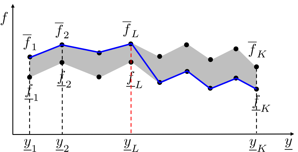
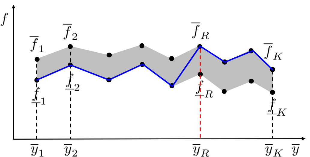
Illustration of the switch points $L$ and $R$ in computing $y_l$ and $y_r$, respectively. (a) Computing $y_l$: the used firing level in $(9)$ switches from the upper firing level to the lower firing level, shown as the blue curve; (b) computing $y_r$: the used firing level in $(10)$ switches from the lower firing level to the upper firing level, shown as the blue curve.
D. Example of IT2 TSK Fuzzy System
Example of IT2 TSK Fuzzy SystemThis subsection uses the car following example again to illustrate the computations in an IT2 TSK fuzzy system.
Assume the distance has three linguistic terms (modeled by IT2 fuzzy sets), Close, Okay and Far, as depicted in Figure $10(a)$, and the relative speed also has three IT2 linguistic terms (modeled by IT2 fuzzy sets), Slow, Okay and Fast, as depicted in Figure $10(b)$. Note again that the word "Okay" for the distance and the relative speed has different IT2 fuzzy set representations.
Figure10(a) Figure10(b)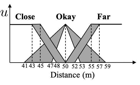
IT2 fuzzy sets for the distance and the relative speed, in the car following example.
There are again nine rules, whose consequents are intervals:
- $\widetilde{R}_1: \mbox{ IF distance is Close AND relative speed is Slow, THEN acceleration is } Y_1=[-1,1]$
- $\widetilde{R}_2: \mbox{ IF distance is Close AND relative speed is Okay, THEN acceleration is } Y_2=[-6,-4]$
- $\widetilde{R}_3: \mbox{ IF distance is Close AND relative speed is Fast, THEN acceleration is } Y_3=[-11,-9]$
- $\widetilde{R}_4: \mbox{ IF distance is Okay AND relative speed is Slow, THEN acceleration is } Y_4=[2,4]$
- $\widetilde{R}_5: \mbox{ IF distance is Okay AND relative speed is Okay, THEN acceleration is } Y_5=[-1,1]$
- $\widetilde{R}_6: \mbox{ IF distance is Okay AND relative speed is Fast, THEN acceleration is } Y_6=[-4,-2]$
- $\widetilde{R}_7: \mbox{ IF distance is Far AND relative speed is Slow, THEN acceleration is } Y_7=[9,11]$
- $\widetilde{R}_8: \mbox{ IF distance is Far AND relative speed is Okay, THEN acceleration is } Y_8=[4,6]$
- $\widetilde{R}_9: \mbox{ IF distance is Far AND relative speed is Fast, THEN acceleration is } Y_9=[-1,1]$
Assume the current distance to the front car is 47 meters, and the relative speed is 4 KM/h. Let $\underline{\mathrm{Close}}$ and $\overline{\mathrm{Close}}$ be the LMF and UMF of $\mathrm{Close}$, respectively. LMFs and UMFs of other words are denoted in a similar way. The membership grades on the corresponding LMFs and UMFs are shown in Figure $11$:
$\quad [u_{_{\underline{\mathrm{Close}}}}($
$\quad [u_{_{\underline{\mathrm{Slow}}}}($
Figure11
Try to drag the dots to change the distance and relative speed values.
The membership intervals and all subsequent calculations will be updated accordingly.
|
Membership intervals on the IT2 fuzzy sets. For each fuzzy set, the UMF is less saturated, and the LMF is more saturated. (a) Distance is meters, the membership interval on Close is [, ], on Okay is [, ], and on Far is [, ]; (b) Relative speed is KM/h, the membership interval on Slow is [, ], on Okay is [, ], and on Fast is [, ].
The firing intervals of the nine rules are:
| Rule No.: | Firing Interval | $\rightarrow$ | Consequent |
|---|---|---|---|
| $\widetilde{R}_1:$ | $[\underline{f}_1,\overline{f}_1]=[u_{_{\underline{\mathrm{Close}}}}($
$\quad\quad\quad\quad=[$ |
$\rightarrow$ | $[\underline{y}_1,\overline{y}_1]=[-1,1]$ |
| $\widetilde{R}_2:$ |
$[\underline{f}_2,\overline{f}_2]=[u_{_{\underline{\mathrm{Close}}}}($
$\quad\quad\quad\quad=[$ |
$\rightarrow$ | $[\underline{y}_2,\overline{y}_2]=[-6,-4]$ |
| $\widetilde{R}_3:$ |
$[\underline{f}_3,\overline{f}_3]=[u_{_{\underline{\mathrm{Close}}}}($
$\quad\quad\quad\quad=[$ |
$\rightarrow$ | $[\underline{y}_3,\overline{y}_3]=[-11,-9]$ |
| $\widetilde{R}_4:$ |
$[\underline{f}_4,\overline{f}_4]=[u_{_{\underline{\mathrm{Okay}}}}($
$\quad\quad\quad\quad=[$ |
$\rightarrow$ | $[\underline{y}_4,\overline{y}_4]=[2,4]$ |
| $\widetilde{R}_5:$ |
$[\underline{f}_5,\overline{f}_5]=[u_{_{\underline{\mathrm{Okay}}}}($
$\quad\quad\quad\quad=[$ |
$\rightarrow$ | $[\underline{y}_5,\overline{y}_5]=[-1,1]$ |
| $\widetilde{R}_6:$ |
$[\underline{f}_6,\overline{f}_6]=[u_{_{\underline{\mathrm{Okay}}}}($
$\quad\quad\quad\quad=[$ |
$\rightarrow$ | $[\underline{y}_6,\overline{y}_6]=[-4,-2]$ |
| $\widetilde{R}_7:$ |
$[\underline{f}_7,\overline{f}_7]=[u_{_{\underline{\mathrm{Far}}}}($
$\quad\quad\quad\quad=[$ |
$\rightarrow$ | $[\underline{y}_7,\overline{y}_7]=[9,11]$ |
| $\widetilde{R}_8:$ |
$[\underline{f}_8,\overline{f}_8]=[u_{_{\underline{\mathrm{Far}}}}($
$\quad\quad\quad\quad=[$ |
$\rightarrow$ | $[\underline{y}_8,\overline{y}_8]=[4,6]$ |
| $\widetilde{R}_9:$ |
$[\underline{f}_9,\overline{f}_9]\quad=\quad[u_{_{\underline{\mathrm{Far}}}}($
$\quad\quad\quad\quad=[$ |
$\rightarrow$ | $[\underline{y}_9,\overline{y}_9]=[-1,1]$ |
Using EIASC, the type-reduced output is computed as:
$ Y($
Finally, the crisp output of the IT2 TSK fuzzy system is:
$ y =\frac{y_l+y_r}{2} =[($
Note that this output is different from the output of the T1 fuzzy system in Section II-C; however, the output of the T1 fuzzy system, $y(47,4)$ in $(4)$, is included in the output interval of the IT2 fuzzy system, $Y(47,4)$ above.
For clarity, the nine rules are also summarized in Table $3$. The corresponding input-output mapping is shown in Figure $12(a)$, which can be changed by modifying the rule consequents in Table $3$. The input-output mapping of the IT2 fuzzy system is more complex than its T1 counterpart in Figure $6$, as evidenced by the difference between their input-output mappings in Figure $12(b)$. Observe also that Figure $12(b)$ looks smoother than Figure $6$, suggesting that the IT2 controller will provide a smoother ride.
Rulebase of the IT2 TSK fuzzy system in the car following example. The intervals are rule consequents, i.e., acceleration (KM/h$^2$). Any interval, as long as the left end-point is smaller than or equal to the right end-point ($\underline{y}_i\leq \overline{y}_i$), can be used for rule consequent, and the IT2 TSK fuzzy system can always give an output. However, The suggested range of each end-point is [-10, 10]. For reasonableness, the rule consequents in the same row should increase from the left to the right, e.g., when Distance is Close, as Relative Speed increases, Acceleration should become more negative, i.e., $\underline{y}_1\leq \underline{y}_2\leq \underline{y}_3$ and $\overline{y}_1\leq \overline{y}_2\leq \overline{y}_3$. The rule consequents in the same column should increase from the top to the bottom, e.g., when Relative Speed is Slow, as Distance increases, Acceleration should also increase, i.e., $\underline{y}_1\leq \underline{y}_4\leq \underline{y}_7$ and $\overline{y}_1\leq \overline{y}_4\leq \overline{y}_7$.
| Distance$\setminus$Relative Speed | Slow | Okay | Fast |
|---|---|---|---|
| Close | $Y_1=[\underline{y}_1,\overline{y}_1]=$ $[$ $,$ $]$ |
$Y_2=[\underline{y}_2,\overline{y}_2]=$ $[$ $,$ $]$ |
$Y_3=[\underline{y}_3,\overline{y}_3]=$ $[$ $,$ $]$ |
| Okay | $Y_4=[\underline{y}_4,\overline{y}_4]=$ $[$ $,$ $]$ |
$Y_5=[\underline{y}_5,\overline{y}_5]=$ $[$ $,$ $]$ |
$Y_6=[\underline{y}_6,\overline{y}_6]=$ $[$ $,$ $]$ |
| Far | $Y_7=[\underline{y}_7,\overline{y}_7]=$ $[$ $,$ $]$ |
$Y_8=[\underline{y}_8,\overline{y}_8]=$ $[$ $,$ $]$ |
$Y_9=[\underline{y}_9,\overline{y}_9]=$ $[$ $,$ $]$ |
Figure 12
(a) Input-output mapping of the IT2 fuzzy system; (b) difference between the input-output mappings of the IT2 fuzzy system and the T1 fuzzy system. The figure can be zoomed and rotated by using the mouse or the top right buttons.
E. Fuzzy System Optimization
IT2 Fuzzy System OptimizationA fuzzy system should be optimized for each specific task. For example, in the car following fuzzy controller, for fast and accurate response, the input membership functions and/or the rule consequents may need to be tuned.
Generally, there are three different strategies
-
Evolutionary computing
. The antecedent and consequent parameters are encoded as chromosomes in a population; genetic operators, e.g., selection, crossover, mutation, and reproduction, can then be used to generate the next (better) generation. The best chromosome in the final generation is selected as the best parameter set.
-
Gradient descent.
For example, back-propagation
can be used to iteratively find the optimal antecedent and consequent parameters. Recently, inspired by the equivalence/similarity between TSK fuzzy systems and neural networks and mixture of expert models , effective optimization techniques for the latter have been extended to fuzzy system optimization . -
Gradient descent and least squares estimation.
For example, in adaptive-network-based fuzzy inference system (ANFIS)
, the antecedent parameters are optimized by gradient descent, and the consequent parameters by least squares estimation.
There are generally two different strategies for optimizing an IT2 fuzzy system:
Evolutionary computing
For example, genetic algorithms, particle swarm optimization , and their combination , have been used. Gradient descent
For example, gradient descent has been used to optimize self-evolving interval type-2 fuzzy neural networks, and a hybrid of decoupled extended Kalman filter and gradient descent has been used to optimize interval type-2 intuitionistic fuzzy logic systems .
F. Main Differences between IT2 and T1 Fuzzy Systems
Main Differences between IT2 and T1 Fuzzy SystemsA challenging question is: What are the main differences between IT2 and T1 fuzzy systems? Once
the differences are clear, we can better understand the advantages of IT2 fuzzy systems and hence better
make use of them. In the literature there has been considerable efforts devoted to answering this challenging and
fundamental question. Some important arguments are
-
An IT2 fuzzy set can model inter-personal uncertainties, which are intrinsic to human language, because its membership is an interval, instead of a crisp number in a T1 fuzzy set. For example, different people may have different understandings of the linguistic terms (Close, Okay, Far, Slow, Okay, Fast) in the car following example, and hence they may provide different T1 fuzzy sets for each word. An IT2 fuzzy set can be used to aggregate the T1 fuzzy sets from different people.
-
IT2 fuzzy sets reduce the rulebase size
, as each IT2 fuzzy set models more uncertainties than a T1 fuzzy set, so that the input/output domains can be covered by fewer fuzzy sets. -
An IT2 fuzzy controller gives a smoother control surface than its T1 counterpart, especially in the region around the steady state (e.g., when both the distance and the relative speed approach 0, in the car following example)
. The Proportional-Integral (PI) gains of the IT2 fuzzy controller also change with the inputs, which cannot be achieved by the baseline T1 fuzzy controller.
Wu
Conclusion
ConclusionFuzzy sets are suitable for modeling human linguistic uncertainties, and the resulting fuzzy systems can
then be used to perform inferences based on a linguistic rulebase. This paper has introduced the basic concepts
of T1 and IT2 fuzzy sets and systems, and illustrated their computations using a car following example.
Fuzzy systems have been used in numerous applications, particularly controls, from cement kiln in Denmark
to Sendai Subway in Japan, from rice cookers to air conditioners. Researchers who want to learn more about
T1 and IT2 fuzzy sets and systems are suggested to read